1Learning Outcomes
Explain how element-wise vector addition and element-wise vector multiplication are SIMD operations.
Understand that SIMD ISAs are extensions of base integer/floating-point ISAs.
🎥 Lecture Video
In this section we discuss SIMD instructions (Single-Instruction, Multiple Data), sometimes known as vector instructions. While we will not build a SIMD architecture, we will see how a programmer can use a SIMD architecture to improve performance.
2Data-Level Parallelism
SIMD architectures exploit Data-Level Parallelism (DLP) with simultaneous operation on multiple data streams. Instead of doing math on one number at a time, SIMD instructions instead do math on several numbers at a time, in a single clock cycle.
SIMD Addition: Figure 1 compares SIMD addition to scalar addition. On the scalar side, we fetch one add instruction and apply it to one pair of operands, A and B. On the SIMD side, we do a vector add: we stil fetch one add instruction, but now we perform vector addition, element by element, for both of the vectors A and B. For the eight-element vectors in Figure 1, vector addition therefore performs one addition (“single instruction”) on eight pairs of operands (“multiple data”) .
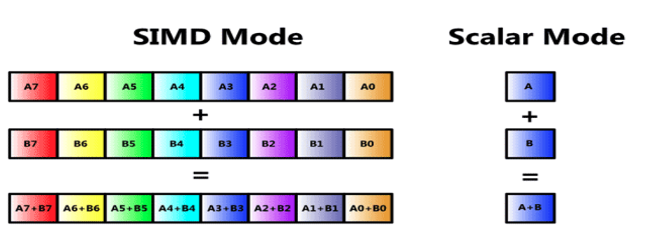
Figure 1:(left) SIMD addition; (right) Scalar addition.
SIMD multiplication: A common vector operation is to multiply some coefficient vector c by some data vector x, element-wise. While this can be accomplished in scalar mode with loops (Figure 2), vector multiplication would again load in one multiplication and apply it to multiple pairs of operands within vectors.
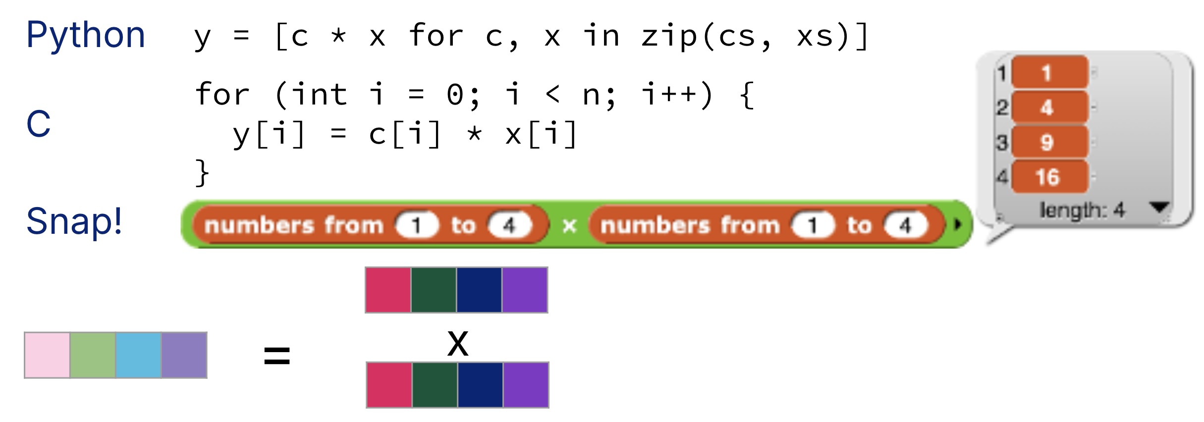
Figure 2:(left) SIMD multiplication; (right) Scalar multiplication.
3SIMD Architecture History
Vector architectures and SIMD architectures[1] have existed for a long time. The first noted SIMD machine was the TX-2 at MIT Lincoln Lab in 1957. The TX-2 had the ability to run full 36-bit-wide data, split it into two 17-bit operands, or split it into four nine-bit operands.[2]
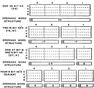
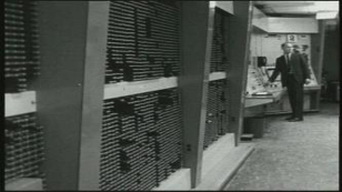
Figure 3:First SIMD Extensions: MIT Lincoln Labs TX-2, 1957.
4Intel SIMD Architectures
SIMD architectures saw wide commercial use when they were introduced on Intel computers in the late 1990s.[3] At the time, more consumers were running more multimedia applications on PCs[4]. These audio and video applications necessitated media applications, which typically involves one-dimensional vectors or two-dimensional matrices.
As a result, SIMD architectures were implemented that performed operations like those in Figure 5. These operations would have two source operands in wide registers, apply the operation to these wide registers, then write the result to a destination wide register.
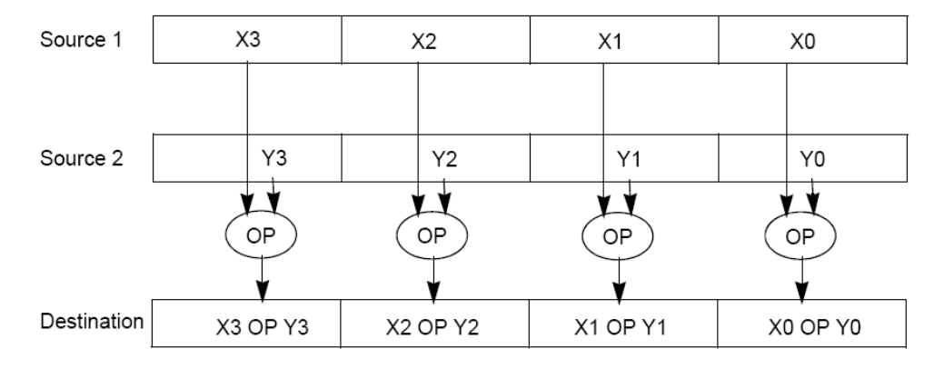
Figure 5:SIMD operands: two source SIMD register operands, one destination SIMD register. If the source registers pack four values of equal width, then the destination register similarly packs four values of the same width.
4.1Intel SIMD ISAs
Intel SIMD instruction set architectures (ISAs) are extensions to the base Intel x86/x87 architecture. The naming of Intel SIMD extensions has changed with functionality. Every few years, there are new instructions, wider registers, and more parallelism.
Figure 6 shows different Intel SIMD ISAs over time.
MMX (Multimedia Extension) was the first SIMD extension on 64-bit registers in Intel’s Pentium 2 Processor (1997).
SSE (Streaming SIMD Extension) uses 128-bit registers and first appeared in Pentium 3 and 4 (1999-2000).
AVX (Advanced Vector Extension) uses 256-bit registers and first appeared in 2011.
AVX-512 uses 512-bit registers and is found in the most recent Intel processors.
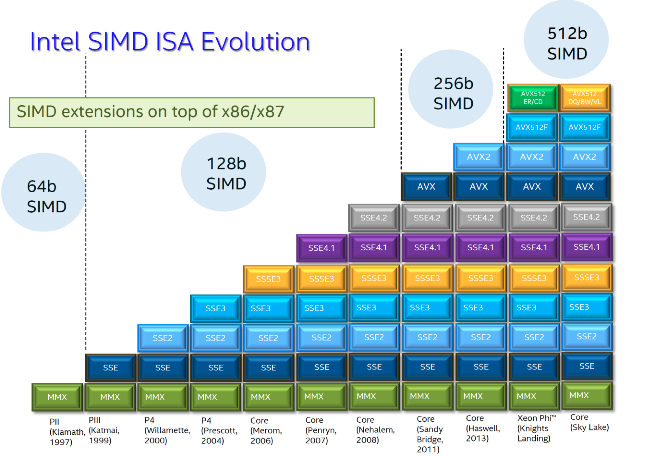
Figure 6:Intel x86 SIMD Evolution: SIMD extensions on top of x86 and x87 (floating point).
All Intel processors are backwards compatible, so even older SIMD extensions like MMX are still around with us. We will see how this complicates documentation for Intel intrinsics.
SIMD architectures and vector architectures are different, but the distinction is beyond the scope of this course. For those curious, most modern vector architectures support a “reduce-add” operation, which sums the elements of a vector together to a scalar result. SIMD architectures do not support such scalar result operations. From Wikipedia: “Pure (fixed-width, no predication) SIMD is often mistakenly claimed to be ‘vector’ (because SIMD processes data which happens to be vectors).”
Remember, standardized bytes/words wasn’t around back then.
See: Intel Advanced Digtal Media Boost from 2009.
Personal Computers, not program counters.